Wednesday October 27th 2004
Finance : Third lecture (part one).
Recall the big objective of
Finance
The three levels at which we are studying finance
Real life financial situations
Risk aversion
Computer
generated simulations of random variables
Definition of
the variability of a random variable : the variance
Notation
Standard deviation
Properties of variance and standard deviation
Exercises
Comparing two securities
Real life securities
Recall the big objective of Finance : How to transform money now, into more value now ?
One thing we know is that we cannot just keep it as is. Money does not grow. We must invest it into something.
We have the choice between totally sure investment, and in financial markets there is only one : purchase of short term government bonds ; or more risky investment, either directly into projects, or indirectly into financial securities.
The objective of Finance can also be expressed in a more technical way : Evaluate the value today of future amounts of money to be received, particularly when these future amounts of money are not sure.
When the future amounts of money are sure, we are not exactly in a finance situation, but rather a case of money management. We know that a sure future cash flow F to be received in one year is worth today F / (1 + r0) where r0 is the rate of return offered by the monetary authorities, in charge of the money we are dealing in, for short term government bonds.
The uncertainty of usual future amounts of money to be received is modelled using the apparatus of probability theory.
The three levels at which we are studying finance
Our study of finance tries to combine progress in our knowledge at three levels :
- real life financial situations and investment opportunities that we can read about in the newspaper : investments in one technology rather than another one, investment into a "sexy" stock, the relative values of various currencies, etc.
- the theory of finance with abstract securities or project investments, random cash flows, profitabilities, optimization of portfolios, etc.
- simple simulations of random variables and securities using a spreadsheet with a random number generating function
Real life financial situations :
Yesterday's paper is quite interesting. For instance the dollar is losing value against the euro. It reached 1,28 dollars for one euro (almost the highest exchange rate reached by the euro, which was 1,29). This rate is due to the uncertainty felt by the international community about the soundness of the American economy.
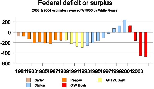
The US federal budget deficit and the US balance of trade deficit (the so-called "twin deficits" because they are of similar sizes) are huge. If the actual president is re-elected they are unlikely to be reduced.
Therefore the US government debt, which is already $7400 billion, is likely to increase further.
Other uncertainties loom over the American economy : like in most western countries, the US social security system is not soundly financed, and it is likely to be bankrupt in one generation. (The problem is particularly acute in France. Since WWII, each working generation is also supplying the retirement income of the preceding generation. This is called an "intergenerational solidarity based system", as opposed to a "capitalization based system" . As long as France population was growing, due to a high rate of new births, this worked fine. But now the demography of France is such that in the coming years, following the retirement of the baby-boomers, there will be less people working and more people retired.)
Bush and Kerry have different economic programs as well as political programs. There is a debate whether Bush managed the economy well or not. His opponents point out the fact that he is the first president since Coolidge, during whose mandate the number of people holding a job decreased. His supporters, on the contrary, say that Bush administration had to face the recession following Internet bubble's burst, the 09/11 attack, and the Iraq war, and yet managed to maintain a high growth rate of the economy.
Anyhow, at some point in the future holding dollars, or dollar denominated bonds, may no longer be a safe way to store value. We only touch on these subjects here, because they will be treated in more depth in the course in International finance, next semester.
We can also read in yesterday's paper that the competition between the three technologies of paying TV, namely cable TV, satellite TV, and DSL Internet TV, is turning to the advantage of DSL Internet TV (for instance, in Europe, via Internet with a high throughput connexion, you can watch CCTV-4 Chinese TV, moreover that one is free).
Suppose a friend of yours invites you to invest into a new venture resting upon a hypothesis of development of satellite TV, and explains to you : "you invest today 100 million €, and next year you get 60 million € and the following year you get another 60 million €". Even though it looks like you can transform quickly 100 million € into 120 million €, you may think that the proposed investment is too risky. If the investment were absolutely sure, it would be a fantastic deal : the value today of 60 million € in one year would be 60 / (1 + 2%) = 58,8 million ; and the value today of the further 60 million € in two years would be 60 / (1 + 2%)2 = 57,6 million €. This yields a total present value of 116,4 million €.
But in truth, the proposed investment is far from an absolutely sure investment. At best the given figures are the mean values of highly speculative cash flows. So the future cash flows must be highly discounted to evaluate their value today. The cash flow projections that are presented to us may also be only the upside of forecasts, or they can be plainly wrong. Anyhow, you should have cold feet.
If you think that this investment is too theoretical, "classroom like", read about the Iridium satellite project, or about the Globalstar project.
There is a fourth future TV in France, called TNT (Terrestrial Numerical Television). But it might also not be such a good bet. Remember : an investment is always a kind of bet.
Today's lecture is devoted to studying how to find and how to use the proper discounting rate to evaluate a proposed investment.
Finally, we can read about Google stock. August 18th 2004, Google floated new stocks on the stock market at a price of $85 per stock. It raised $1,67 billion dollars of fresh money for Google. The shares rose 18 percent to $100 on their first day of trading. Now, three months later, the same stocks are traded on the stock market at a price of $185. "Financial analysts" were quite critical of the initially contemplated introductory price of $125, later on revised to $85. Now they "forecast" a future price of $200 "in 12 to 18 months"...
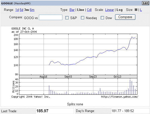
Source : http://finance.yahoo.com/
Google is very exciting. But remember, it is also very risky. The leading engine before Google, around 5 years ago, was Altavista. Who uses Altavista today ?
In order to make up your mind about the future of Google stock price you will have to pore over their management, their past achievements, their projects... So far it looks like Google is much better managed than Altavista was. Altavista first belonged to Digital Equipment Corporation, then when DEC hit big problems Altavista was divested (i.e. sold). Then it did not receive the amount of managerial and financial resources necessary for its development. And now it's too late.
Another well known stock market success story is Microsoft.
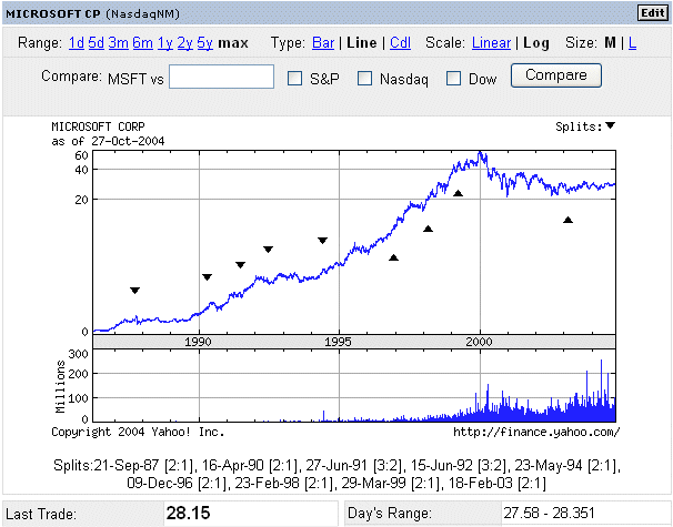
People who bought Microsoft shares when there were initially issued in 1986 multiplied their investment about 300 times. (Use the historical data, for instance on http://finance.yahoo.com/, specifying all the stock splits to get the exact figure.)
Then the question is : "Will Google be a future Microsoft, or a future Altavista ?" We could also mention Netscape as a "child prodigy project" that didn't keep up with promises.
What can be said today is that Google is much better managed than Altavista was, and that it is seriously gearing up for the big fight with Yahoo and Microsoft for the control of a large market share of the future technologies of finding, shaping and catering information. For instance Google is contemplating creating its own browser. And Google has a good track record of innovations of all sorts in the information business (see http://www.google.com/options/index.html )
e-Bay (the online auction service) is also one the current stars of the stock market. Thousands of people in the US earn their living exclusively using e-Bay. e-Bay recently acquired the Internet banking service Paypal. You should read about all these stories.
Amazon is another, somewhat older, high-tech venture on the Net (at the beginning, an online bookstore) the story of which is also worth studying. It consumed large amounts of money during its first years, that Amazon's founder, Jeff Bezos, had to explain were investments and not plain losses. Now it seems like Amazon has, at last, achieved financial viability, but it was everything but a easy bet.
This year, you must read business newspapers several times a week.
After these three examples from real life financial situations, let's go back to more theoretical considerations : that is the second category of finance studies we conduct.
Finance people are risk-averse. By this we mean precisely the following : When finance people are offered for purchase two securities, S or T with the same expected cash flows in one year, they will offer a higher price for the security the random cash flow in one year of which has less variability.
S is a security promising an amount of money X in one year. T is a security promising an amount of money Y in one year. X and Y are random variables. And E(X) = E(Y). Then financiers prefer the security S if and only if
variabiliy of X is less than variability of Y
Otherwise they prefer T.
So we have to define more precisely what we mean by "variability" of a random variable.
So far I casually said "it is the dispersion of the possible values of the random variable", but now we need a clear, precise definition.
In order to build up our intuition and feel for randomness, random variables and their various characteristics, we will turn to the third type of finance studies : simple simulations generated using a computer.
Your job, as students learning Finance, is to always keep in your mind the links between the three types of finance studies we conduct.
Computer generated simulations of random variables :
With the help of Excel we can generate numbers ui's selected at random between zero and one, with a uniform density of probability.
In other words we can generate as many outcomes as we like of a random variable U, uniformly distributed between zero and one. For any segment [a, b] contained in [0, 1]
Pr{ a ≤ U < b } = b - a
Let's understand this well : the outcomes of U are chosen between 0 and 1, with no area of the unit segment more likely to contain the outcome than others. This is a very simple and natural continuous RV.
With Excel the function to produce a random outcome uniform between 0 and 1 is "=RAND()"
(Type this formula into a cell, without the quotes, and see the result. To update, that is produce another outcome in the same cell, press F9.)
Such a computer-generated random variable is very convenient to study all kinds of discrete RV (and also continuous RV but we shall leave this aside).
For example in lesson 2a we studied a wheel with sectors producing a random payoff X taking the possible values
a1 = $70
a2 = $80
a3 = $100
a4 = $110
a5 = $115
with the following probabilities
Pr{X = a1} = 30°/360° = 8.33%
Pr{X = a2} = 70°/360° = 19.44%
Pr{X = a3} = 120°/360° = 33.33%
Pr{X = a4} = 60°/360° = 16.67%
Pr{X = a5} = 80°/360° = 22.22%
From U it is simple to produce a random variable that behaves exactly like X :
draw an outcome u1 of U between 0 and 1
then to u1 associate a value x1 (that is called "a fonction of u1") defined a follows
if u1 is less than 8.33%, then x1 = $70
if u1 is greater than 8.33% but less than 8.33% + 19.44% (=
27.77%) , then x1 = $80
if u1 is greater than 27.77% but less than 27.77% + 33.33% (=
61.10%) , then x1 = $100
if u1 is greater than 61.10% but less than 61.10% + 16.67% (=
77.77%) , then x1 = $110
and finally
if u1 is greater than 77.77% , then x1 = $115
To produce a series of outcomes of X we just reproduce the process.
Here is a result with 5796 replications of "spinning the wheel" and producing a payoff :
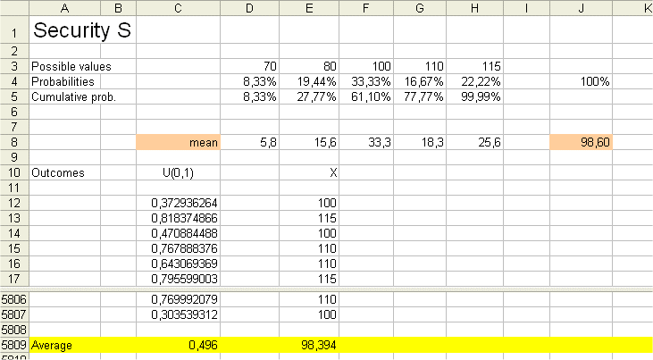
The sheet contains the calculations of the exact Expected value of X, this is the weighted average of the possible outcomes weighted with their probabiliies. The result is E(X) = $98.6, as we already calculated in lesson 2.
But this sheet also contains 5796 outcomes of X (x1, x2, x3, ...................., x5796).
And we computed their simple average. The result is $98.394
This result is not far from E(X) as we know it should be.
Definition of the variability of a random variable :
To define the variability of X we will use probabilistic characteristics of the deviation of each outcome from the mean E(X).
The deviation of outcome x12 from the mean is
x12 - E(X)
Since this number can be positive or negative and we want a positive figure, be x12 bigger or smaller than E(X), we square this deviation.
We could use absolute values like | x12 - E(X) | because these also are always positive quantities, but it turns out that the mathematics are simpler to handle with squared deviations. In some esoteric space, we can define length of RV in relation to these squared deviations, and the Pythagoras theorem applies for "orthogonal" RV. Orthogonality for RV will be independance. We shall study, using intuitive tools and simple maths, dependance and independance of RV later.
The series of squared deviations are
(x1 - 98.6)2, (x2 - 98.6)2, (x3 - 98.6)2, .............................................. (x5796 - 98.6)2
These are outcomes of the random variable [X - E(X)]2
By definition the variance of X is the expected value of [X - E(X)]2
Variance(X) = E{ [X - E(X)]2 }
After some practice this complicated looking object will become natural and simple. Here is its computation with our Excel sheet.
It is simple to compute the expected value of [X - E(X)]2 , because it is a random variable that can take only five values with the same five probabilities as X itself. So computing its mean is easy.
The result is 217.5
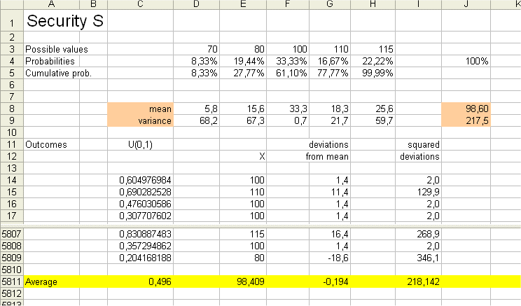
Furthermore, we have an estimated figure for this average squared deviation. We obtain it from averaging the outcomes of it from the 5796 replications of "spinning the wheel". (Caveat : it is a new batch of 5796 replications from above.)
We get the estimated variance 218.142. This is not far from the exact variance 217.5. Everything is fine.
The variance of X is denoted σ2X
Or, when there is no ambiguity, σ2
By definition the standard deviation of a random variable is the square root of its variance.
Here standard deviation (X) = square root of 217.5 = 14.747
The standard deviation of X is denoted σX
Or when, there is no ambiguity, σ
Properties of variance and standard deviation :
Variance of ( X + constant ) = Variance of X
because adding a fixed number to X doesn't change its variability.
Variance of ( aX ) = a2 times Variance of X
Therefore standard deviation of ( aX ) = a times ( std dev of X )
Note, for later on, the following consequence :
standard deviation of [ ( X - P ) / P ] = ( std dev of X ) / P
that is the standard deviation of the profitability of the security S is equal to ( std dev of random cash flow of S) / P
1) Compute with a hand held calculator the mean and variance of a random variable Y taking the following values
| Possible values | 60 | 70 | 80 | 110 | 126,5 | ||
| Probabilities | 5% | 10% | 20% | 50% | 15% | ||
Answer :
| mean | 100,0 |
| variance | 405,3 |
2) Compute with a hand held calculator the mean and variance of a random variable Z taking the following values
| Possible values | 60 | 70 | 90 | 130 | 155 | ||
| Probabilities | 5% | 15% | 50% | 20% | 10% | ||
Answer :
| mean | 100,0 |
| variance | 747,5 |
Suppose the RV Y above is the random payoff in one year of a security T, and Z above is the random payoff in one year of a security V.
As you can see, the two securities were constructed to have the same expected payoff, $100.
But the variability of the payoff of V is much higher than the variability of the payoff of T.
The stock market will give a higher price to T (the less risky security) than to V (the more risky security)
For instance T will sell for $80, and V will sell for only $70.
That way, the expected profitability of T will be ( 100 - 80 ) / 80 = 25%
And the expected profitability of V will be ( 100 - 70 ) / 70 = 42.9%
This is an illustration, with a made up example, of a general rule we already saw, and we repeat here :
The market adjust prices so that riskier securities yield higher profitability.
So far we have created discrete securities, equivalent to wheels with sectors, to study their probabilistic and financial characteristics.
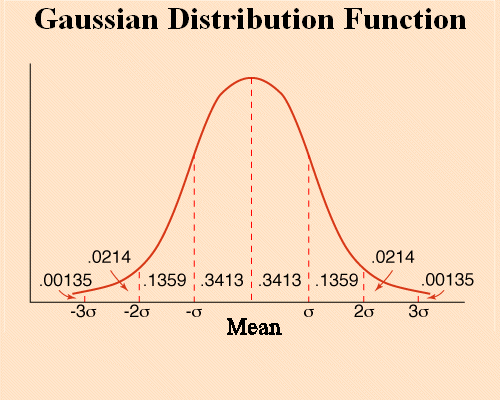
In real life the securities we shall encounter will be such that their random payoffs will be more or less Gaussian distributed.
And therefore their profitability will also be Gaussian distributed. That is with density of probability like this :