Finance with a review of accounting

discounted cash flow analysis, and introduction to joint random variables

Cost of equity : the formula r = (D1/E) + g

    when we exchange give out a sum of money E (ie we buy equity) in exchange for a stream of future CF [D1, D1(1+g), D1(1+g)², etc.] our investment has an IRR which is called the cost of equity, because it is what the investor expects from the firm issuing stocks.

Cost of debt

Weighted Average Cost of Capital (WACC)

The Polyzone example

Now we want to turn to optimizing a portfolio of securities. This will be explained in detail here : Joint random variables

But let's take a look at the simple underlying ideas :

So far we studied one random variable X, produced by an experiment E, sometimes in a very general probabilistic setting, sometimes we specified that it was the profitability of a given security S which we buy today and will sell in one year. The experiment E here is : "Wait one year from today". And at the end of that year, we sell S, make a profit or a loss, and we compute the profitability yielded by S.

(We include in our profit the possible dividends produced by S.)

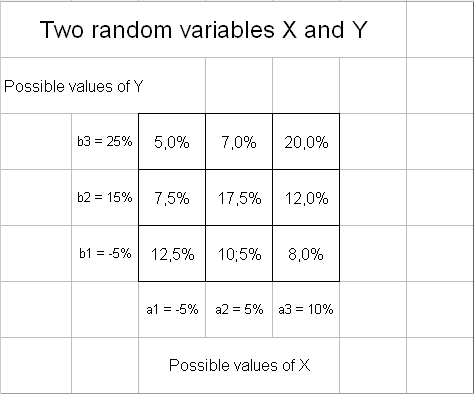
But in the stock market (think, for instance, of the New York Stock Exchange), if we perform the experiment "Wait one year", many random variables will have an outcome, namely the profitability of each and every securities we can buy today on this market, and sell in one year.

We want to invest into a bunch of securities to form a portfolio. So we need to study several random variables produced at the same time in one experiment "Wait one year". We shall start with two random variables: X and Y (think of them as the profitabilities over the year to come of IBM stock, and Microsoft stock).

And to make life simple, assume that X can take values in a finite set of values {a₁, a₂, ... a_n}, and Y can take value in a finite set of values {b₁, b₂, ..., b_m}. If we make these two sets rich enough, we can always produce a quite acceptable approximation of real life securities.

Now the pair (X, Y) can take values in the set obtained by crossing {a₁, a₂, ... a_n} with {b₁, b₂, ..., b_m}. We usually picture it as an array of possible pairs :

For each of these pairs there is a probability : p_ij  also naturally displayed in an array.

Example :

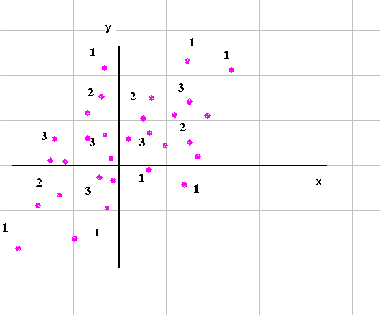
And if we produce a long series of outcomes of (X, Y)

(x₁, y₁), (x₂, y₂), (x₃, y₃), ... ... ... , (x_{10 000}, y_{10 000})

each outcome will fall in one of the n times m cells above.

On top of that, the frequency of each possible pair will be a good approximation of the probabilities.

All this is a pure extension of what we studied for one RV.

The name, in two dimensions, corresponding to the one dimensional histogram, is the "scattergram". Here is an example (with the count of pairs of outcomes in each cell of the grid) :

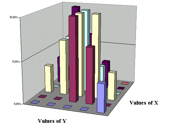
or, represented in 3-D,

There is one new concept (explained in detail here :  Joint random variables with the help of a game of guessing the outcome of X) : it is the concept of relationship between X and Y. Sometimes we shall say that X and Y are independent, and sometimes we shall say that X and Y are dependent.

In the above examples, they are dependent : if we try to guess the outcome of X, having information on the outcome of Y helps sharpen our guess on X.

We shall compute a "covariance" of X and Y, which will measure the extend to which the outcome of one is related to the outcome of the other.

Next to the covariance of X and Y, we will compute another measure (very close in concept) called the correlation of X and Y.