Wednesday 27th October 2004

Finance : Third lecture (part two).

Price, future cash flow and profitability of a security S
Why are we more concerned with r than with E(X) or P ?
Simulation of S with price 5€ and profitability 20%
Risk aversion of investors, and profitabilities
The fundamental fact of Finance
One more reason why it is the profitability that matters
The sequence of yearly prices of a security is a random walk
What happens when the profitability has little variability
The limit case of fixed profitability
Example of real securities
Calculating the price of T when we can buy a security S that has the same risk pattern
Verification that a higher price P_T would not be acceptable to an investor
Definition of the opportunity cost of capital
The traditional (σ, r) graph where we position securities

Price, future cash flow and profitability of a security S

As regards investing into a security, in Finance we are more interested in the profitability of the security than in the absolute value of its price or of its future cash flow.

Remember the three quantities related to a security S :

P = price of S today

X = future value of S in one year (and therefore future cash flow of money, if we were to sell S in one year). X is a random variable

R = the (unknown today) profitability of S. So R is also a random variable.

They are linked by the following equation :

R = (X - P) / P

When it is necessary to avoid ambiguity, we denote these quantities

R_S,   X_S   and P_S

If, following usage, we denote r = Expected value of the random profitability of S, then we also have

r =  ( E(X) - P ) / P

or equivalently

P = E(X) / (1 + r)

Usage often calls "profitability of S" what is actually the "expected profitability of S". Usually we know from context what the authors mean, but still we always have to be careful.

Why are we more concerned with r than with E(X) or P ?

Let's take a simple example : consider a security whose price P is 5€, and expected payoff in one year is E(X) = 6€, then its profitability (that is, to be more accurate, its expected profitability) is r = 20%.

But for us, as investors, the actual price and expected cash flow of S don't matter much. What matters is its profitability.

Indeed if we want to invest 1000€, we just buy 200 securities S, and we expect to have in one year 1200€ of worth.

We have the same profitabiliy r = 20% than with just one security.

People who, last August, invested into Google stock did not invest $85 into one Google share. Some people invested $1000, and some other invested $10000 or more. (In fact there was so much anticipated demand that Google management rationed - i.e. restricted to limited allotments - the number of shares one investor could buy, but that's another story.)

Altogether Google stock float brought $1.6 billion of fresh money to the firm from tens of thousand new stockholders, but not from 19 million new investors.

What matters today to Google recent investors is not so much the two figures "today's price is $190" and "issuing price was $85", as the fact that "in three months, the price was multiplied by 2.24".

Simulation of S with price 5€ and profitability 20%

In order to get a better feel for the security S let's simulate S using the random number generator of Excel.

S has an expected payoff in one year of 6€. And today it costs 5€. Therefore its average profitability is 20%.

The payoff next year is a random variable. That is that we can think of many replications of "the experiment producing the future payoff of S" and think of the many different outcomes we would get.

With Excel we can generate a Gaussian random variable X with mean 6.

We also have to decide which variance σ², or equivalently standard deviation σ, we shall give to X. Let's choose σ = 1.333...€

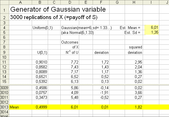
Here is a possible sequence of 3000 outcomes of X :

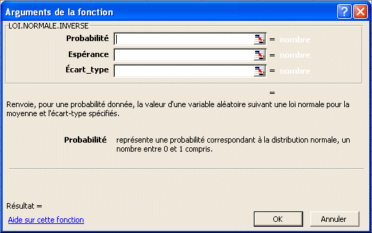
I used the function "=RAND()" for the uniformly distributed U(0,1), and I transformed it into a Gaussian(6 ; 1.333) using the function "=inverse normal distribution"

This sequence of 3000 outcomes of X is

 7.72€,  7.43€,  7.17€  ...  ...  ...  4.09€,  5.48€

We know that the exact mean of X is 6€

and the exact standard deviation is 1.333...€

And we can, with satisfaction, see that the average of the 3000 outcomes X of  is 6.01€, and the estimated standard deviation (that is the square root of the average squared deviation) is 1.35€.

This simulates 3000 possible outcomes of X, the payoff of S in one year.

This simulation should help us feel the randomness of the future payoff of the security S.

Caveat : these do not simulate a sequence of prices from one year to the next (see below) but what the price next year could be. A sequence of yearly prices is a slightly different concept : it is a random walk. We shall see below what is meant by that.

As we saw, what really matters to investors is the expected profitability of S (often, abusively, called "the profitability of S"). So let's show the profitability of S. Here is a (new) batch of 3000 outcomes of S :

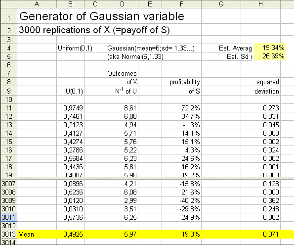
Now, we display the profitability corresponding to each outcome of X. The first outcome of X is 8.61€, so the first instance of profitability is (8.61-5)/5 = 0.722, or equivalently 72.2%.

The whole sequence of profitabilities is

72.2%,  37.7%,  -1.3%, ... ... ... -29.8%,  24.9%

These are outcomes of the random variable R = (X - P)/P.

We know that the exact mean of the random variable R is 20%, and the exact standard deviation of R is 1.33€.../5€ = 26.66...%

And we can observe that the estimated mean of R from this second batch of 3000 outcomes of X is 19.34%, and the estimated standard deviation is 26.69%.

As we know, for investors these two numbers are important : the average profitability of S (20%) tells them that they can expect a gain of 20% on their investment into the security S. They can invest into one S if they want. This costs 5€. But nobody does that. They will rather invest into 200 or 2000 S's and expect to gain 20%.

(Note that in the US stock markets most stocks have a price of the order of magnitude of $100. And in the UK it is typically around 1£.)

The second number, the standard deviation, is quite important too. It tells investors what is the variability of the profitability they will get.

Risk aversion of investors, and profitabilities :

We already saw that investors are risk averse (it can be formalised using the theory of utility, initiated by Daniel Bernoulli). Let's see very precisely what this entails.

We need to go back to the absolute figures of the future cash flows paid by S and by T. As usual we call them X and Y.

If investors are offered two securities S and T for purchase, with the same expected cash flows E(X) = E(Y), but different standard deviations σ_X and σ_Y, with say  σ_X < σ_Y, then they will prefer the security S. By this we mean that the price of S on the market will be higher than the price of T.

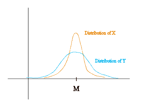
Let's call M the common mean of X and Y.

We know that the prices P_S and P_T are both less than M. (No investor will pay for a security more the its expected value in one year. Only gamblers do that.)

From the investor's risk aversion behavior we see that P_S > P_T

Then necessarily

[E(X) - P_S]/P_S < [E(Y) - P_T]/P_T

because of the shape of this function (use for instance the free little software called Power Toy Calculator, distributed by Microsoft, to draw this graph) :

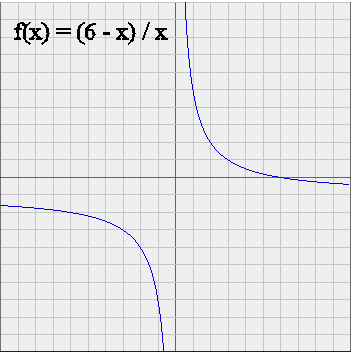
Put another way, the expected profitability of S is less than the expected profitability of T :

r_S < r_T

This is a fundamental fact of Finance :

when two securities promise the same average payoff in one year, the riskier one (the one whose payoff is more variable) has a higher profitability.

One more reason why it is the profitability that matters :

We already saw that investors will not pay much attention to the actual price of a security S. What matters to them is the profitability they can expect. So whether the stock trades for 5€, 20€, or 85€ does not really matters, as long as it can be expected to bring a profitability r.

We saw that S will produce a random payoff X, and we simulated many outcomes of the future payoff of S to get a feel for it.

These outcomes of X do not simulate a sequence of values of S over several years. They simulate outcomes of the value of S next year, if we could "reproduce" the occurence of next year many times.

Indeed from one year to the next the price of S varies. What, one year n, is the future value X that will be observed year n+1, becomes, next year, the new price of S. So the values of S over many years are not independent instances of one random variable. But the sequence of observed profitabilities r₁, r₂, ... r_n,... from one year to the next is a sequence of outcomes of one random variable R.

This is one more reason why in Finance we deal with profitabilities, their mean, and their standard deviation, more than with absolute price and cash flow of securities.

The sequence of yearly prices of a security is a random walk :

Let P₁, P₂, P₃, .... P_n, P_n+1, ... be the prices of a security S over a series of years (for simplicity we consider a security with no dividend, for instance the corresponding firm reinvests whatever profit it makes).

Then, any given year n, the price of the security is P_n, and, viewed from that year, the future value X is precisely what will become next year price, that is P_n+1

So we have

P_n+1 = P_n times (1 + r_n)

where r_n is the profitability of investing into S at year n.

The sequence of P_n's are not outcomes of a single RV, but the sequence of r_n's are outcomes of a single random variable R, with a mean r and a standard deviation σ.

Here is a graph of the sequential prices of S for a security that begins at 5€, and the profitability of which from one year to the next is a RV with mean 5% and standard deviation 20% :

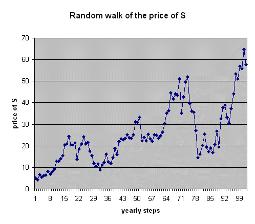
The sequence of 100 yearly profitabilities is :

-13%,   +52%,   -15%,  ....   +16%,   -11%

The mean of this series is 5%, and the variability of the profitabilities around their mean, measured by the square root of the average squared deviation, is 20%.

Exercise : Use the simulation tool put on the website to observe the behavior of many random walks with exactly the same probabilistic characteristics. The results you'll get may not be as your intuition suggests

Here is the histogram of 100 outcomes of R :

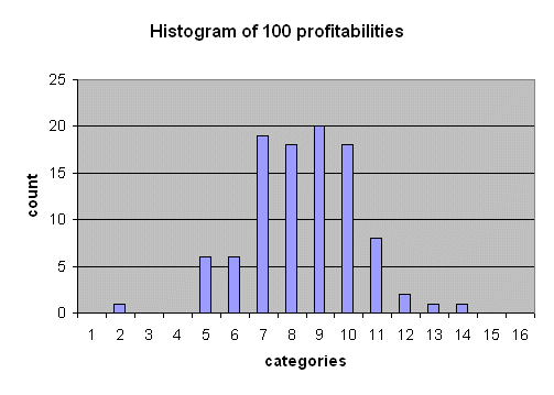
the categories are the following percentages :

To sum up :

The yearly profitabilities are independent outcomes of a Gaussian random variable with mean r and standard deviation σ. In the above example r = 5% and σ = 20%.

And the actual prices follow a random walk generated by the equation

P_n+1 = P_n times (1 + r_n)

The above graph shows a typical such random walk.

What happens when the profitability has little variability :

When the profitability R has little variability around its mean, the random walk of the prices of S has quite a different look.

Here is an example with r = E(R) = 5%, but σ is small : σ = 5%.

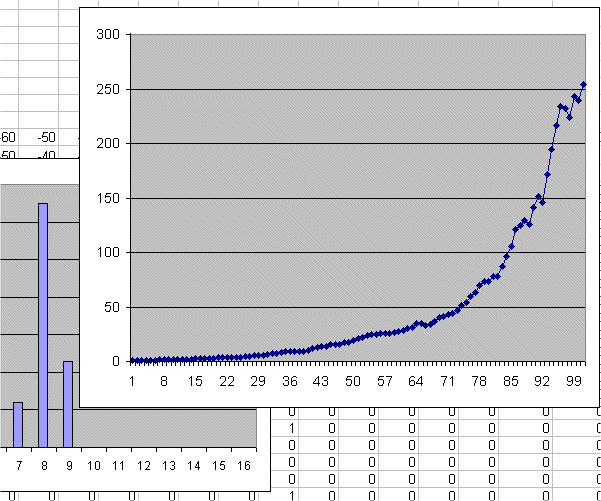
We see the histogram of the 100 years of profitability, and the random walk of the prices of S.

It is not surprizing that the random walk begins to look like an exponential.

Indeed from a price P_n on year n, the next price P_n+1 has little randomness because r_n has little randomness.

r_n is almost equal to 5% every year. So the prices that are linked by the relationship

P_n+1 = P_n times (1 + r_n)

are almost linked by P_n+1 = P_n times (1 + 5%), which is the equation of an exponential growth.

The limit case of a fixed profitability :

The limit case of a fixed profitability from one year to the next is an old friend of ours : it is when we lend money to a risk free borrower.

This is when, and only when, we purchase government bonds of rich "safe" countries.

We know that in today's markets we cannot get a risk free rate of 5% !

In the US the risk free rate in October 2004, for lending dollars, is 1.75%. And in the Euro Zone, for lending euros, it is 2%.

If we were to lend a sum of money P for 100 years at the fixed rate of 2% per year, we would get at the end of the period

P₁₀₀ = P times (1 + 2%)¹⁰⁰

(1 + 2%)⁴ = 1.0824

(1 + 2%)³² = 1.8845

(1 + 2%)⁶⁴ = 3.5515

So (1 + 2%)¹⁰⁰ = 7.2443

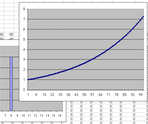
Lending 1€ for one hundred years at a yearly rate of 2%, with no variability in this factor, yields 7.24€ at the end of the period.

And this can be seen from our random walk simulations as well, were we set E(R)=2% and σ_R = 0. It is no longer properly speaking a random walk, because each step is just a multiplication of the previous price by 1 + 2% :

Example of real securities

The prices of real securities are modelled as random walks, at least on "reasonably short" periods of time (periods going from a few weeks up to a few years, when no "structural reason" changes the behavior of market prices).

In the first part of this lecture we saw the price of Google stock since last August :

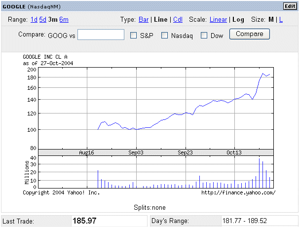
This graph has a logarithmic vertical scale, to represent on the same graph small figures as well as large figures.

Many financial analysts think that this is essentially a random walk. To go from the daily price one day to the price of the next day, a multiplication by (1+Rd) takes place, where Rd is the profitability over one day. It is a random variable with a certain mean and variance, that can be estimated from the 100 or so past figures available.

That is how "in the short term" (a few days to a few weeks) future prices can be forecast.

In the longer term, there often are "extra causes" that "explain" big variations, that are not just "randomness at work". The whole point of financial investments analysis is to figure out these "extra causes".

More "exotic" securities can also be studied, like the price today of contracts for future delivery of orange juice in three months :

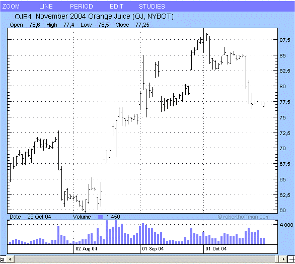
Source : http://futures.tradingcharts.com/

In the short term we still have just instances of random walks.

Calculating the price of T when we can buy a security S that has the same risk pattern :

Consider two securities S and T, that promise cash flows X and Y.

Suppose we know E(X), σ(X), E(Y) and σ(Y).

We say that S and T have the same risk pattern iff, up to a possible rescaling factor, X and Y have the same probabilistic behavior. If they have the same risk pattern then

E(X) / σ(X) = E(Y) / σ(Y)

(or equivalently σ(X)/E(X) = σ(Y)/E(Y)  )

For instance a security S promising 6€ in one year, with a standard deviation of 1.333...€, has the same risk pattern as a security T promising 180€ with variability 40€. For financial investors S and T are equivalent.

So if, on the market, S trades today for 5€, that is has an average yield r_S = 20%, then necessarily on the market today T trades for a price P_T that also yields a profitability of 20%. So the following relation must hold

By rewriting differently this relation, we obtain the fundamental equation of Finance : it gives the price that T must have :

Pay close attention to this equation : it gives the price today of T by dividing the expected cash flow of T in one year by (1 + the profitability of S). (We call this operation "discounting E(Y) by r_S".

With the above numerical figures, this gives P_T = 150€.

Verification that a higher price P_T would not be acceptable to an investor :

S and T have the same risk pattern. Their future payments are respectively 6€ and 180€, with standard deviations 1.333...€ and 40€.

And S yields a profitability of 20€, that is S sells today for 5€.

Suppose that T is offered for a price higher than 150€, say it sells for 160€. Let's see that this is not an acceptable price for an investor.

Suppose the investor buys one security T at a price of 160€. Then he will receive in one year a value Y whose expected value is 180€, so his investment has a profitability 20/160 = 12.5%. This is less than investing into S.

And the standard deviation of the profitability of his investment is σ(Y)/160 = 40/160 = 25%.

This is also less than the standard deviation of the profitability of S, which is 1.333.../5 = 26.67% But it does not qualify investing into T as an acceptable investment, because we can make the following investment instead : invest 150€ into buying 30 S's and keep the extra 10€ as is. Call this "investing into V".

The expected profitability of V is 30/160 = 18.75%

And standard deviation of profitability of V = 30 * 1.333 / 160 = 25%

In other words, V is indisputably superior to T : same risk 25%, and higher profitability, 18.75% instead of 12.5%.

So T sold at a price of 160€ will never be bought by an investor.

The technique of creating a new security by combining two types of investment (here S and something very simple : keep your money)  is a common technique in Finance to establish various results. We shall meet it again.

Definition of the opportunity cost of capital :

When we are considering a possible investment J into a security or into a physical project, if we have the possibility to make other investments or to invest into other securities, which have the same risk pattern as J and the profitability of which is are known figures, then the maximum such other profitability is called "the opportunity cost of capital of the investment J".

This heavy sounding definition is really quite natural : when we invest some money into a project J, we give up the opportunity to invest the same money elsewhere ! So the profitability of the investment we give up is some sort of cost to us. It is called "the opportunity cost of capital".

In the preceding section, T and S had the same risk pattern and the profitability of S was known to be 20%. So we required to pay for T a price that brought at least this profitability.

We computed P_T as :

where E(Y) is the expected cash flow T will produce.

In other words,

to compute the value today (P_T) of an investment (buying a security T, or more generally investing some money today) we discount its future cash flow in one year by its opportunity cost of capital.

The traditional (σ, r) graph where we position securities :

Securities traded in the stock market have two important characteristics : their expected profitability r , and the standard deviation of their profitability σ.

We saw above (at the beginning of this second part of the lecture) that these two characteristics are more important to investors than their actual price and future cash flow.

r is customarily, and slightly abusively, called "the profitability of S"

σ is the financial definition of "the risk of S".

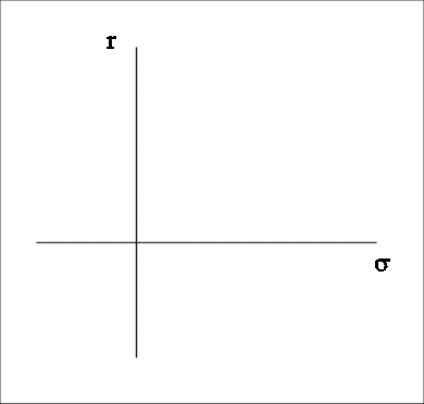
Securities are often positioned on the following graph :

Go to lesson 4