Wednesday January 12th 2005
Finance : twelfth lecture (part one)
Portfolios of securities (cont'd)
Introduction
Exercise
Estimations of joint probabilities
The role of intuition in scientific creation
Estimations of joint probabilities (cont'd)
Securities in the market are positively linked
Covariance and correlation
Properties of covariance and correlation
Geometric interpretation of correlation
Calculation of covariance and correlation in an example
Exercise
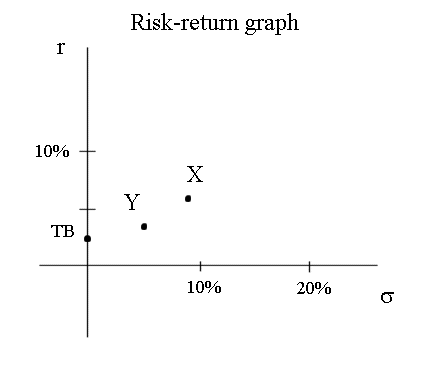
Position of X and Y on the risk return graph
We continue studying investments into portfolios made of several securities. When we have money which we want to invest into the stock market, we usually don't want to invest it all into one security, but we prefer to invest it into a portfolio made of several securities.
This requires to study collections of random variables produced in the same experiment. We say that they are produced "jointly". This is the modelisation of "looking up every day - or every year - the price of every security, and therefore the profitability of every security, in the newspaper", and "see how our investment into several stocks is doing".
The random variables we study are the profitabilities of different securities we can buy in the market.
The concepts introduced last time and today will enable us to calculate the profitability and the risk of portfolios, and to sort out good portfolios and bad portfolios.
Exercise :
Suppose X and Y are random profitabilities with the following joint distribution :
| Y | ||||||
| 10% | 0% | 0% | 5% | 5% | ||
| 5% | 5% | 15% | 15% | 5% | ||
| 0% | 5% | 15% | 15% | 0% | ||
| -5% | 5% | 5% | 5% | 0% | ||
| X | -10% | 0 | 10% | 20% |
In red are the possible values which X can take and whichY can take. We have denoted them earlier a1, a2, a3, a4 and b1, b2, b3, b4. And in the 4x4 array are the probabilities of each pair of possible values.
Calculate the mean and the standard deviation of X :
we must first calculate the "marginal distribution of probabilities" of X. They are
Pr{X = -10%} = 15%
Pr{X = 0%} = 35%
Pr{X = 10%} = 40%
Pr{X = 20%} = 10%
To construct an intuitive feeling for probabilities it is often useful to think of a large number of replications of the experiment E producing the outcomes, because then the probability of an event is the same as the frequency of occurence of the event in the long series of replications of E.
For instance if we produce (X, Y) 10000 times, we shall get
(x1, y1), (x2, y2), (x3, y3), ... ... ... (x10000, y10000)
In this large collection of outcomes of (X, Y) there will be 40% (approximately, but rather precisely because we look at a large series of replications of E) of the pairs where xi is 10%.
Then E(X) = a1 Pr{X=a1} + a2 Pr{X=a2} + a3 Pr{X=a3} + a4 Pr{X=a4}
= -10% x 15% + 0 x 35% + 10% x 40% + 20% x 10%
= 4,5%
To compute the standard deviation, we compute first the variance. The variance is the expectation of the squared deviation of X. So we have to compute the four possible squared deviations :
sqdev1 = (a1 - 4,5%)2 = (-0,145) x (-0,145)
= 0,021025
sqdev2 = (a2 - 4,5%)2 = 0,002025
sqdev3 = (a3 - 4,5%)2 = 0,003025
sqdev4 = (a4 - 4,5%)2 = 0,024025
What is the expectation of the squared deviation of X ? It is the weighted mean of these four products, with the four probabilities Pr{X = ai} as weights. (It can also be thought of as the simple average of the 10 000 squared deviations computed from the long series of outcomes above.)
The result is Variance of X = 0,007475
And, therefore, Standard deviation of X = 8,6%
These two numbers, E(X) and σ(X), describe the profitability of an investment into the security X. (Here we assimilate the security and its profitability and denote both X.)
If we have $1000 and invest them into X, next year on average we shall have $1045. But there is a risk : $1045 is only the expected sum we shall have. It can turn out to be more, it can turn out to be less. To simplify the calculations, we have assumed that X can take only four values :
-10%, 0%, 10% and 20%
with probabilities
Pr{X = -10%} = 15%
Pr{X = 0%} = 35%
Pr{X = 10%} = 40%
Pr{X = 20%} = 10%
The standard deviation of our random profitability is 8,6%.
More realistic profitabilities can take a continuum of values and are Gaussian distributed. (But then the calculations require a bit of calculus.)
Calculate the mean and the standard deviation of Y :
similar calculations yield E(Y) = 2,25% and σ(Y) = 4,3%
We note that, if we are in the US stock market, Y is not an interesting security, because it has the same mean as short term Treasury bonds (which are risk free) but it has a risk. So, as we know, investors will prefer TB, and will never invest into Y.
Estimations of joint probabilities :
In the above exercise we have assumed that we knew the theoretical probabilities of (X, Y). It is simpler to begin learning, but it is not the most realistic case.
Remember that we meet probabilities in four different situations :
| We know the theoretical probabilities | We know only a past history of outcomes | |
| Discrete RV | ||
| Continuous RV |
More realistic cases are in the right column. Usually we deal with RV's which are continous in nature, but we round them off, so they behave like discrete RV's.
In the right column, there are two sub-columns :
In the case where we have a long past history of outcomes we are almost back in the left column : if our RV's can take a discrete set of values we can estimate precisely the probabilities with frequencies of outcomes ; if our RV's are continous we can draw histograms or scattergrams which estimate precisely densities of probabilities.
The role of intuition in scientific creation :
Only a good introductory course in Probability can clarify all the questions you may ask yourself on the relationship between theoretical probabilities and estimations from series of past outcomes, or on the relationship between histograms, scattergrams and densities of probabilities. In this Finance course we have only introduced the main elementary concepts and relied much on intuition.
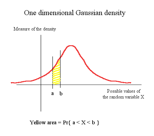
Here is a one dimensional Gaussian density of probability

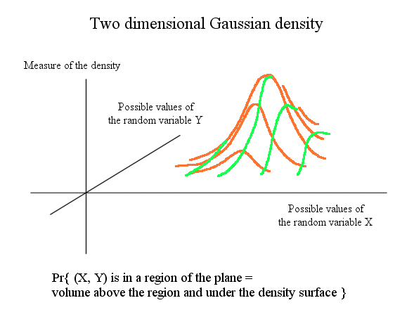
Here is a two dimensional Gaussian density of probability
Remember that it is always intuition - that is comparison of what we are in the course of studying with our past experience, which means : with other mental models we developed when we were younger -, and never heavy manipulation of equations, that is at the heart of creation and discovery. In fact manipulation of equations always comes second, to help clarify intuition - sometimes to correct it - and help go farther in discovery and creation. This will have to be done in Economics and in Money, where current concepts and intuitions are poor, and must be enlarged. But it will be done by first creating new concepts from a larger intuitive view of, for instance, monetary phenomena - that is exchange with the means of various kinds of promises - and second formalizing them with equations. No progress can be achieved by investigating further current models with more equation-cranking ; they have been investigated to the last nook and cranny and have produced all they could. Therefore, tackling the current model of economic exchanges in a community with the usual agents (consumers, producers/firms, bankers, central bank, gouvernment, rest of the world, etc.) and the usual tools (money, credit, currencies, property, etc.) is bound to lead nowhere.
Estimations of joint probabilities (cont'd) :
In the case where we only have a small past series of outcomes we are in the realm of statisticians : they will compute estimates of all sort of things and be quite concerned with the quality of their estimators. We will not be concerned with this situation. We will always assume that either we know the theoretical probabilities, or we can have sufficiently good estimates of them from long past history.
A swarm of dots representing a long series of outcomes of (X, Y) can always readily be transformed into a joint distribution of probabilities. Here is an example :
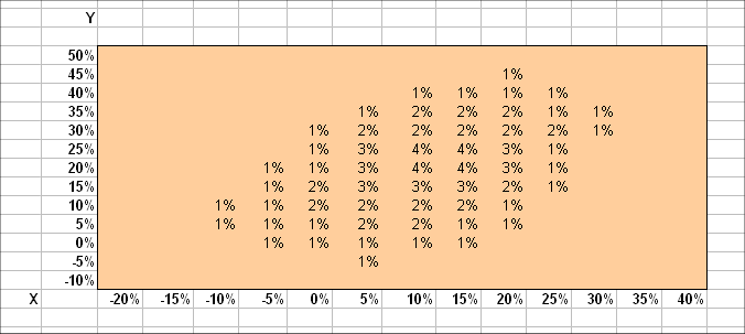
Here X and Y are the random profitabilities of two securities in the stock market. They have been rounded off less roughly than in the first exercise. (They are not the same RV's, even though I use the same letters.) Calculations, here, yield E(X) = 11,1% , σ(X) = 8,7%, E(Y) = 20% and σ(Y) = 10,9%.
Securities in the market are positively linked
Real securities in the stock market are always positively linked. They all move in same direction as the whole market. And each will add some specific randomness on top of the general movement which is itself random.
The link between two random variables is measured by the concept of covariance, and the derived concept of correlation.
The covariance of X and Y is, by definition,
Covar(X, Y) = Expectation { [X - E(X)] times [Y - E(Y)] }
And Correlation (X, Y) = Covar(X, Y) / σ(X) . σ(Y)
Correlation (X, Y) is often denoted ρXY
The correlation of X and Y is just the covariance rescaled by the two standard deviations.
Properties of covariance and correlation
1) Covariance of X and X = Variance of X
2) If we replace Y by a + bY, then the covariance of (X, Y) is just multiplied by b :
Covar (X, a + bY) = Covar (X, bY) = b times Covar (X, Y)
3) Since, for a positive b, σ(a + bY) = σ(bY) = b times σ(Y), then
Correlation (X, a + bY) = Correlation (X, Y)
In other words : A positive linear transformation on one random variable does not change its correlation with another one. A negative one changes only the sign.
4) Correlation (X, Y) is a number always between -1 and +1
5) If X and Y are independent then Covar (X, Y) = 0, and therefore Correlation (X, Y) = 0. This can be proved as a consequence of the fact that if X and Y are independent then
E(XY) = E(X) times E(Y)
And this last result is obvious if we use our usual long sequence of outcomes of (X, Y) to figure it out. From the long sequence (x1, y1), (x2, y2), (x3, y3), ... ... ... (x10000, y10000) let's compute the 10000 products xiyi and add them up. Let's look at the pairs where xi = a1. Suppose there are n1 of them. They will have the yj's with the proportions leading to E(Y). More precisely the n1 products x1yi add up to x1n1E(Y). So the 10000 product xiyi add up to 10000E(X)E(Y).
6) If we work only with Gaussian or approximation of Gaussian random variables (the usual situation in Finance) the converse is true too : if Correlation (X, Y) = 0 then X and Y are independent.
Geometric interpretation of correlation
Correlation = +1
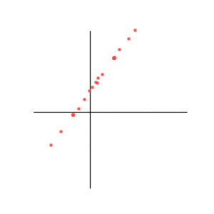
Correlation = + 1
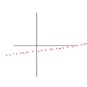
The correlation is +1 if and only if the two variables are linearly related with a positive coefficient : Y = aX + b. The steepness (a) of the slope does not play any role. And the second coefficient (b) doesn't play any role either.
Correlation = -1
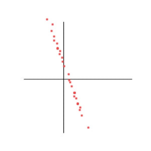
There again the steepness of the slope does not play any role. And a translation of the swarm of points won't change anything either. (The line doesn't have to go through zero-zero).
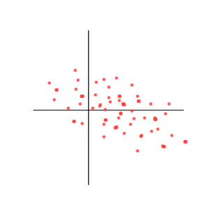
Positive correlation, but less than one
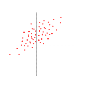
Negative correlation, but more than -1
Correlation = 0
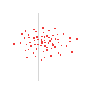
Above we see that there is no relation between X and Y. More precisely, if we are told "what was Y", it does not help us guess "what was X".
Below is displayed a weird situation where Correlation = 0, but the variables are not independent. But their joint distribution is not Gaussian, and doesn't concern us in simple Finance.
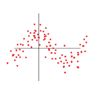
Calculation of covariance and correlation in an example
Let us go back to our first example above :
| Y | ||||||
| 10% | 0% | 0% | 5% | 5% | ||
| 5% | 5% | 15% | 15% | 5% | ||
| 0% | 5% | 15% | 15% | 0% | ||
| -5% | 5% | 5% | 5% | 0% | ||
| X | -10% | 0 | 10% | 20% |
and let's now compute the covariance of X and Y, and then their correlation coefficient.
The covariance of X and Y is the expectation of the product (X - E(X))(Y - E(Y)).
So we have to compute the 16 possible values of this product, and average them with the probabilities as weights.
Product 1 : (-10% - 4,5%)(-5% - 2,25%) = 0,0105125
The frequency of this first product is 5%
Product 2 (moving from a1 to a2, and staying with Y = b1) :
(0 - 4,5%)(-5% - 2,25%) = 0,0032625
The frequency of this second product is 5%
... ... ...
Product 16 : (20% - 4,5%)(10% - 2,25%) = 0,0120125
with frequency 5%.
Sometimes you will see this calculation denoted
Covar(X, Y) = Si Sj (ai - μX)(bj - μY)Pr{X=ai and Y=bj}
The result is Covariance (X, Y) = 0,001488
and Correlation (X, Y) = 39,8%
Compute E(X), σ(X), E(Y), σ(Y), covar(X, Y) and corr(X, Y) with the following data :
| Y | ||||||
| 10% | 0% | 0% | 11% | 10% | ||
| 5% | 5% | 12% | 13% | 6% | ||
| 0% | 8% | 14% | 13% | 0% | ||
| -5% | 4% | 4% | 0% | 0% | ||
| X | -10% | 0% | 10% | 20% |
Answers :
E(X) = 5,2%
σ(X) = 9,54%
E(Y) = 3,5%
σ(Y) = 4,44%
Covar (X, Y) = 0,00248
Corr (X, Y) = 58,5%
Position of X and Y on the risk return graph
