CORPORATE FINANCE
Session 4 : Sensitivity analysis, Simulations
Main textbook for the course : Brealey and Myers, Principles of corporate finance, McGraw-Hill
Sensitivity analysis, Simulations
Let's consider an investment in a project.
We have all the data necessary to do a DCF :
We can compute the NPV of the project, and see whether it is positive or not.
But that is not the end of the story.
We can perform a sensitivity analysis, i.e. let some of the important variables vary and see what happens to the NPV of our project.
Here is an example (chapter 10 of the textbook) :
It concerns a projected investment into a new plant to manufacture electric scooters.
We can right away mention that the revenues we will anticipate will depend upon exogenous variable like the price of oil.
Here are the numbers :
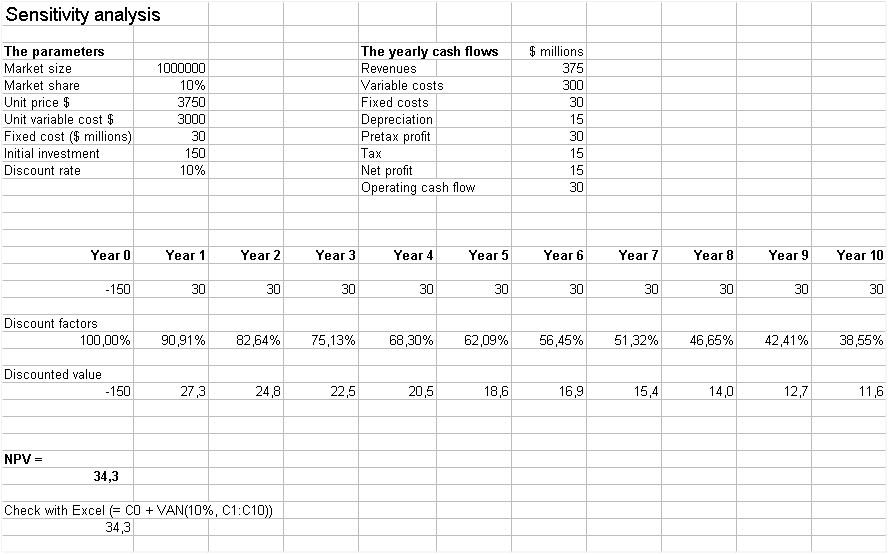
C0 (the initial investment) is US $ -150 million
Then, for ten years, we anticipate the same income structure each year as follows (in millions of US $) :
| Revenue | 375 |
| Variable costs | 300 |
| Fixed costs | 30 |
| Depreciation ($150 depreciated over 10 years) | 15 |
| Pretax profit | 30 |
| Tax (50% of pretax profit) | 15 |
| Net profit | 15 |
| Operating cash flow | 30 |
The DCF analysis of the series of cash flows (discounted at 10%) yields NPV = $34.3 millions.
So everything is fine...
But what are the assumptions under which these figures have been constructed ? Here they are :
Market size : 1 000 000 electric scooters each year
Market share of our venture : 10%, i.e. 100 000 scooters per year
Selling price : well $3750
Variable costs per scooter : $3000
Fixed costs : $30 millions
Initial investment size : $150 millions
The following spreadsheet gives us the possibility to do a sensitivity analysis (called sensitivity_analysis.xls)

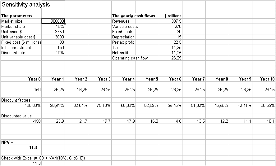
For instance if the market size assumption is changed from 1 000 000 to 900 000, then the NPV becomes $11.3
(see the sheet below) :
Using this spreadsheet we can fill out the following sensitivity analysis table : (or we can use a faster method)
(Here, for the sake of simplicity, we change only one variable at a time)
| Pessimistic | Expected | Optimistic | |
| Market size NPV |
900000 11.3 |
1000000 34.3 |
1100000 57.4 |
| Market share NPV |
4% -103.9 |
10% 34.3 |
16% 172.6 |
| Unit price NPV |
3500 -42.5 |
3750 34.3 |
3800 49.7 |
| Unit variable cost NPV |
3600 -150.0 |
3000 34.3 |
2750 111.1 |
| Fixed costs NPV |
40 3.6 |
30 34.3 |
20 65.1 |
(One more sensitivity trial : if the discount rate is set at 12% then, every else being equal, the NPV becomes $19.5 millions)
From the above tableau, we see which variables play an important role and which variables do not (of course all this depend upon the value we give to these variables in the various hypotheses) :
here the unit cost at $3600 makes the NPV plunge at - 150 millions of dollars
and the market share at only 4% makes the NPV plunge at -104 millions of dollars
Another example of use of the sensitivity analisys, suppose the production dept is worried that the unit variable cost may be 3200 instead of 3000, then the NPV becomes -27.1
(see below)
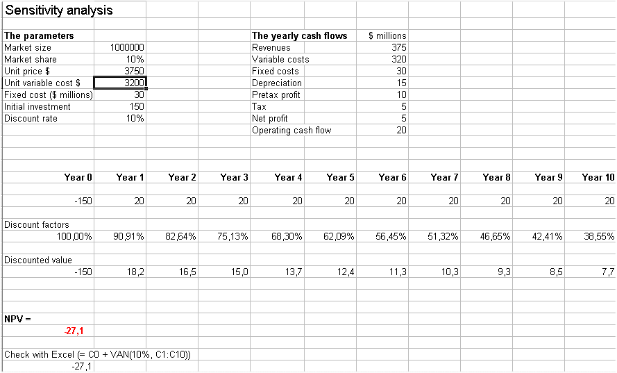
That is the NPV plunges from 34.3 to -27.1 = a plunge of 61.2 million dollars.
Then the production dept adds "we are not sure ; the probability is 10% that the cost will be 3200 instead of 3000 ; a further test costing $100 000 will enable us to check this".
Would you do the test or not ?
Of course sensitivity analysis requires to make hypotheses, "pessimistic" hypotheses, "normal" hypotheses, and "optimistic" hypotheses.
All this is very subjective.
Another approach to sensitivity analysis : Break-even analysis
We are familiar with the notion of break-even point from the technique of marginal costing systems in managerial accounting.
Here the concepts are very similar.
Let's see that with sales :
If sales are zero NPV = -196.1
If sales are 100 000 NPV = 34.3
If sales are 200 000 NPV = 264.8
OK :at what sales number the NPV crosses zero to become positive ?
There are many ways to get at this figure. Interpolation is one. But since we have a spreadsheet a trial and error method (always going in the middle of the values that give positive and negative values) will give us a more precise answer.
It turns out to be : sales = 85100 units -> NPV = 0
We could also draw lines for present value of inflows and present value of outflows at several levels of sales.
Note that when the pretax profits are negative, the tax is negative and becomes an inflow (because the negative profit can partially or totally offset the positive profit of another project)
In fact we find that
sales = 0 -> taxes = -22.5 (negative taxes are a positive "side" cash flow in a DCF analysis, because they can decrease positive taxes elsewhere in the firm)
sales = 100 000 -> taxes = 15
and sales = 200 000 -> taxes = 52.5
A common mistake :
Sometimes managers to find the break even point (in terms of sales) look up when the profit cross zero.
They say "at this level, we will get back our investment so that's OK"
This yields sales = 60 000
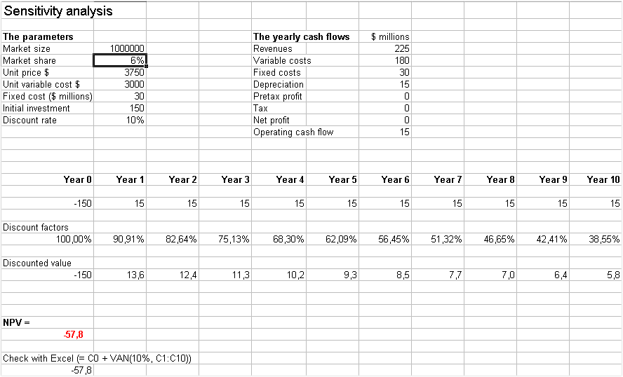
But this is a mistake. The NPV is -57.8
They overlook the fact that future cash flows (of 15) must be discounted with the opportunity cost of capital (here 10%)
$ 150 million today is not equal to a stream of ten yearly cash flows of 15 millions
It is equal (at 10% discount rate) to a stream of ten yearly cash flows of $24.41 millions
That's precisely what yields an NPV of zero, and that is 85100 units sold per year.
There is a famous example, where Lockheed engineers thought the break-even point for a new airplane project (costing $1 billion) was 200 airplanes, when actually it was 500. They had forgotten the opportunity cost of not using $1 billion in another project of the same risk (i.e. they had forgotten the discount rate)
Monte Carlo simulation
The theory and techniques of Monte Carlo simulations were developped by the polish mathematician Stan Ulam (a great mathematician that also invented one of the key devices to make a hydrogen bomb explode).
The basic idea underlying Monte Carlo simulations is somewhat simple :
if a variable V is a function of several variables, X, Y and Z, for instance : V = F(X, Y, Z)
and each variable X, Y and Z is a random variable and therefore (X, Y, Z) is a tri-dimensional random variable
and we know the frequency distribution of (X, Y, Z)
but it is very difficult to compute mathematically the frequency distribution of V = F(X, Y, Z)
then an approximate solution is as follows :
draw a great many outcomes of (X, Y, Z) : (x1, y1, z1), (x2, y2, z2),... (xn, yn, zn)
for each set (xi, yi, zi) compute vi = F(xi, yi, zi)
then the statistical distribution of the vi's is an approximation of the frequency distribution of V
and we did it without complicated mathematical calculations.
This technique can be applied to sensitivity analysis :
Suppose that the parameters of our project are random variables for which we know roughly the frequency distribution.
Then we can compute the frequency distribution of each cash flow C1, C2, C3, etc.
See exhibit 10-5 of the textbook
Then we can compute the expected value of each cash flow
and finally we can do our DCF analysis taking into account this randomness
NPV = C0 + ExpectedC1/(1+r) + ExpectedC2/(1+r)2 +ExpectedC3/(1+r)3 + etc.
Note that an NPV itself is never a random variable : it is one number : the best estimation of the Net Present Value of our project under all the assumptions made including randomness (that lead to cash flows that are random variables : but we use their expected value)